Workflow
Each tool reads the output of the one before it. The flood raster is an input of the first tool, so no label field is needed on your points or grid.
Flood raster and predictor rasters, read at your points or grid cells, written to a CSV.
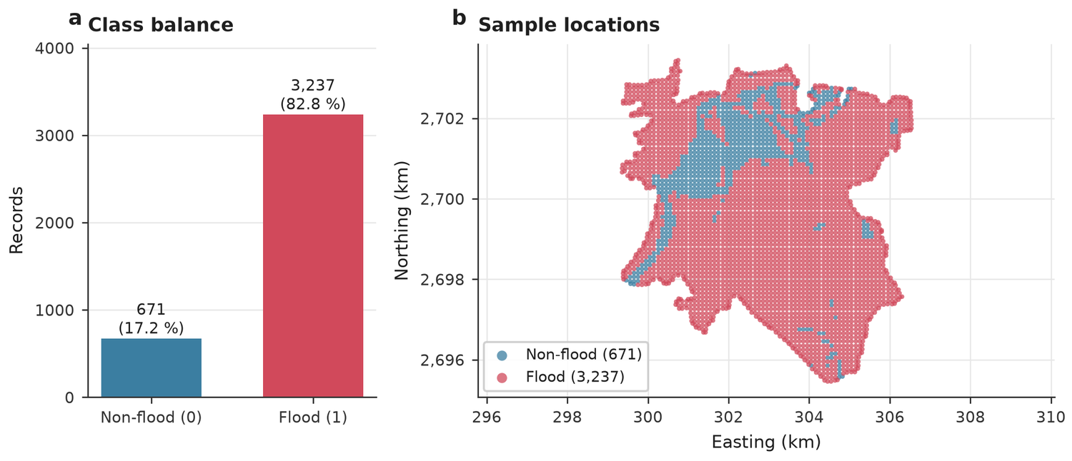
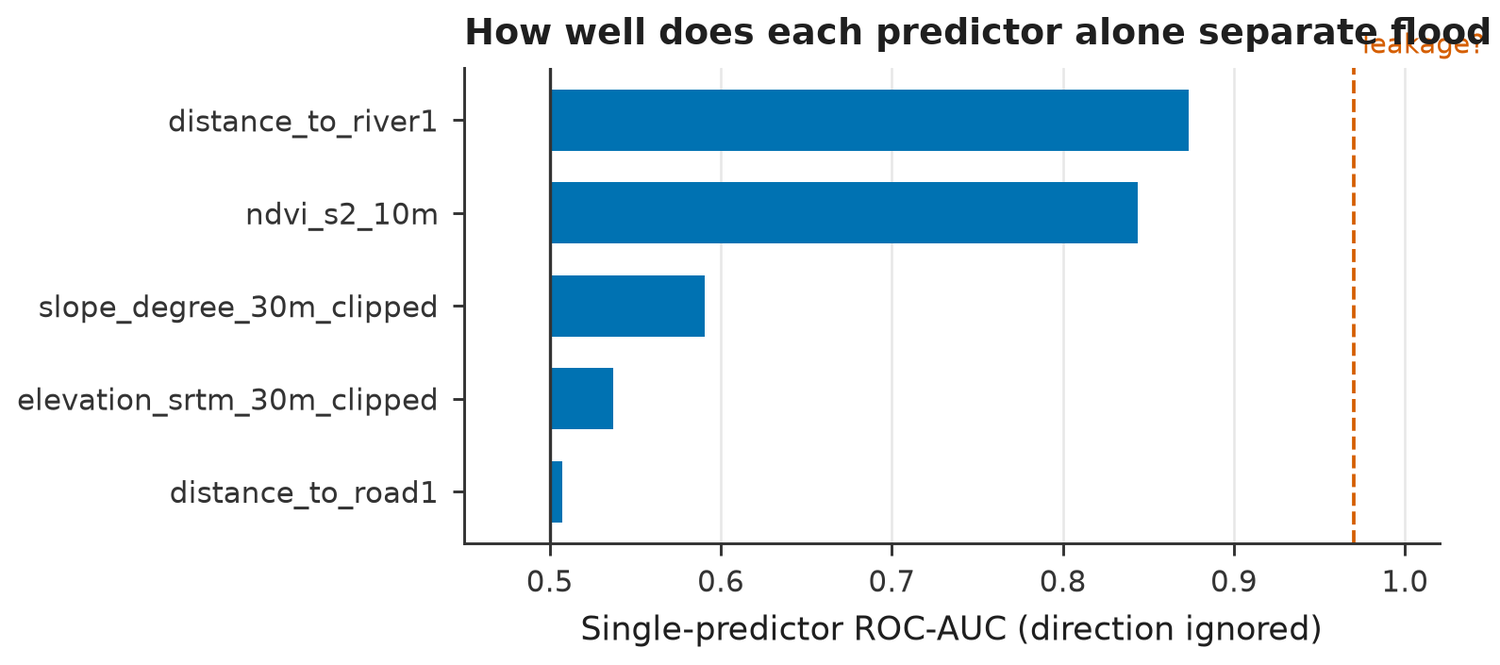
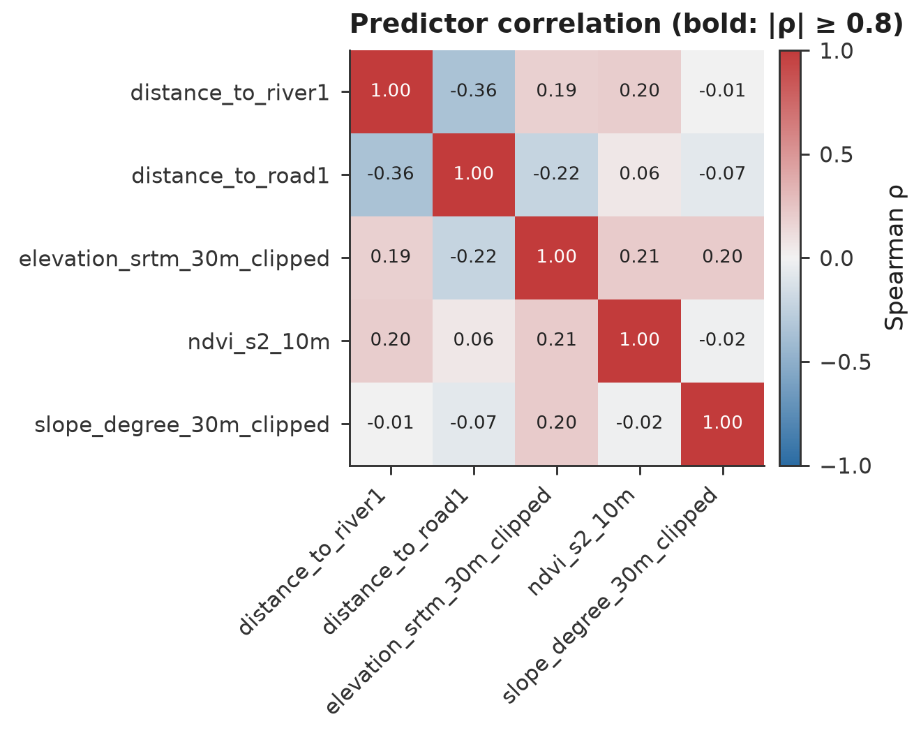
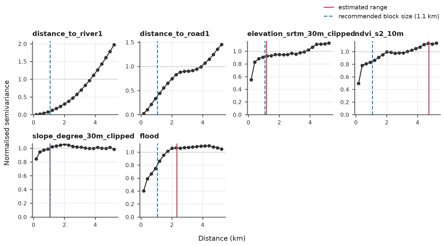
Class balance, leakage hints, correlation and a suggested block size.
Nested spatial cross-validation, confidence intervals, SHAP, residual maps.
Susceptibility raster, classes, styles and an extrapolation warning raster.
Scores on data the models never saw, with an overlap check.
Runs the whole chain on synthetic data and says whether it works.
Susceptibility map
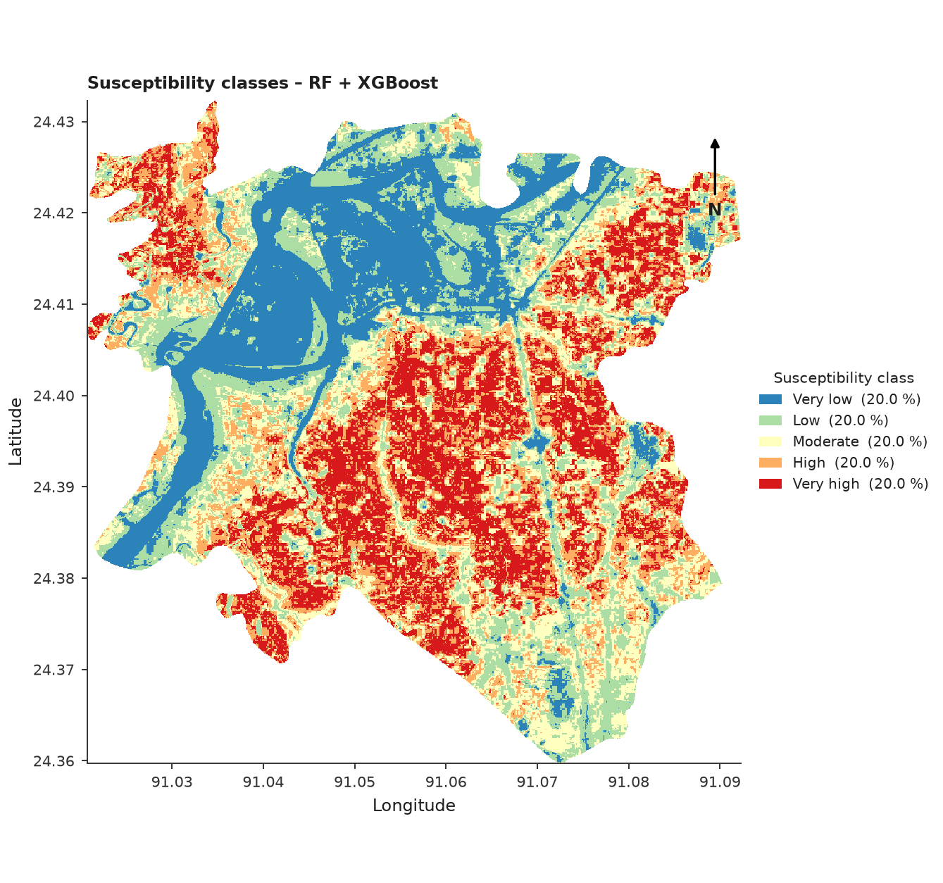
Five classes from the ensemble prediction. With quantile classes each class holds about the same number of cells by design, so the map ranks places against each other. It is not a probability of flooding.
Data check
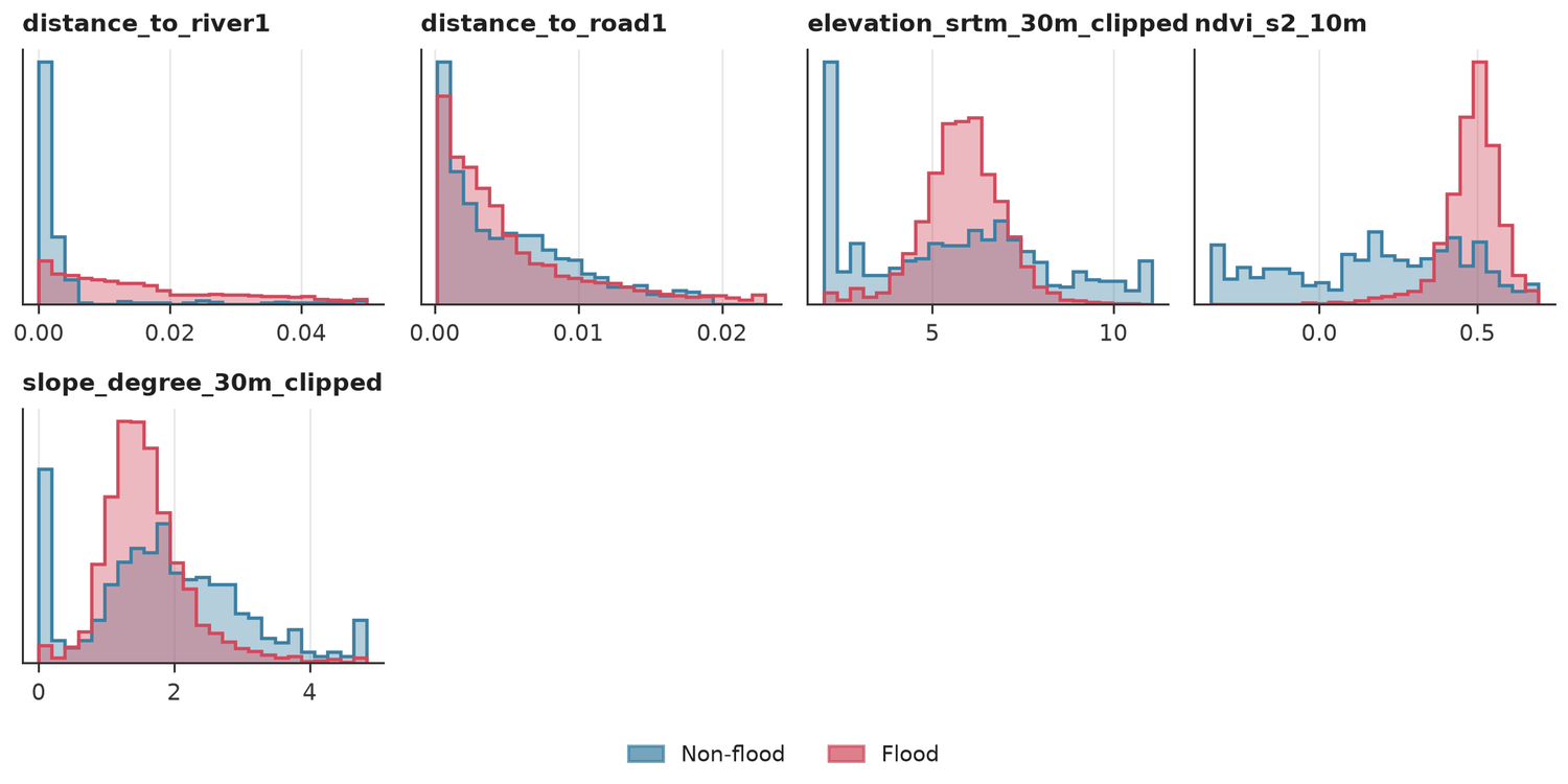
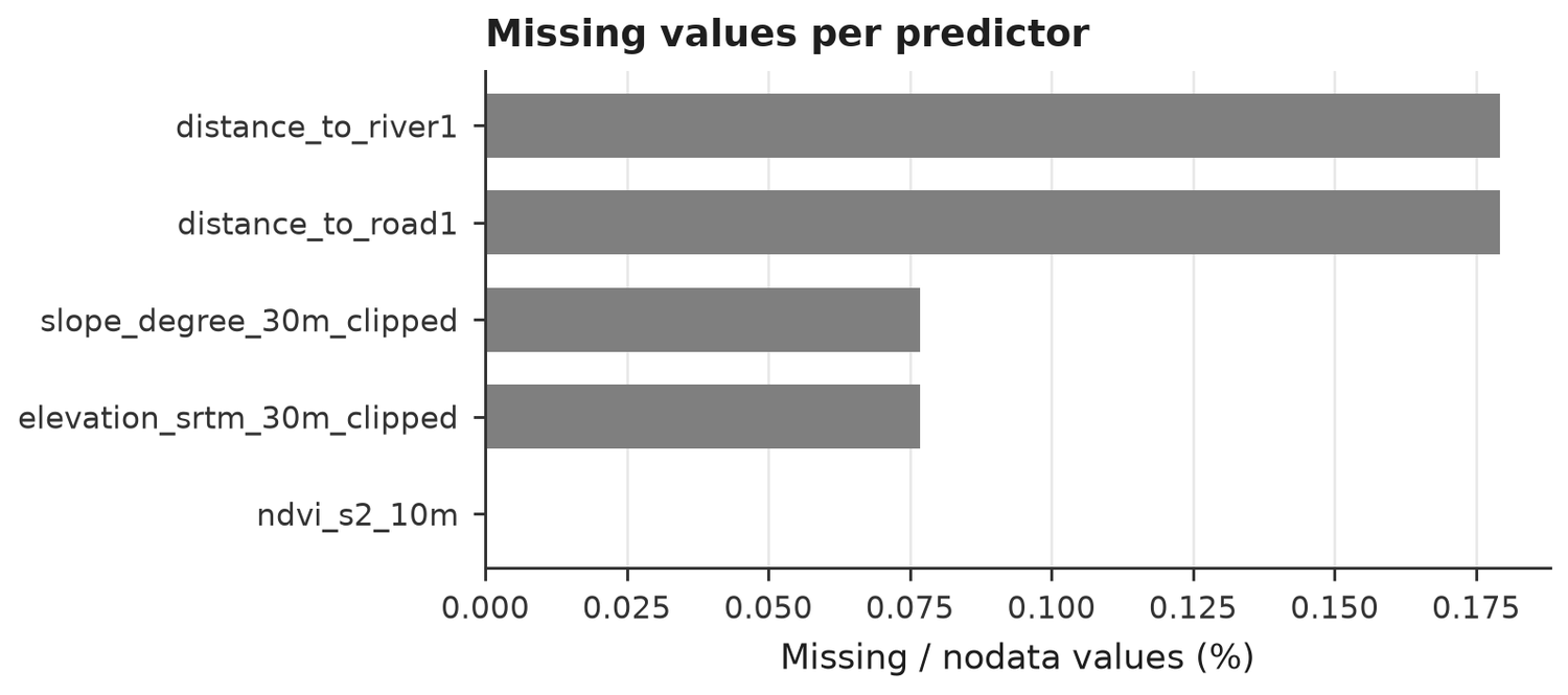
Tool 02 inspects the CSV before any model is trained.
Variance inflation
| feature | vif |
|---|---|
| distance_to_river1 | 1.225 |
| distance_to_road1 | 1.221 |
| elevation_srtm_30m_clipped | 1.162 |
| ndvi_s2_10m | 1.114 |
| slope_degree_30m_clipped | 1.050 |
Spatial validation
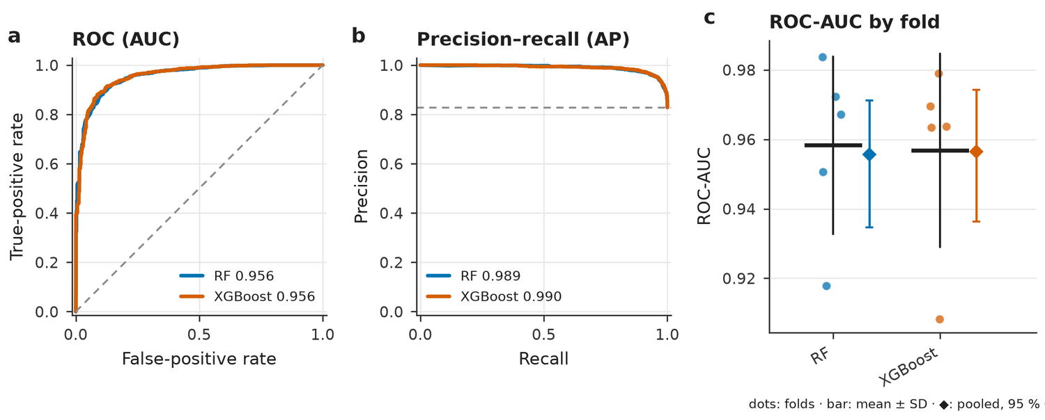
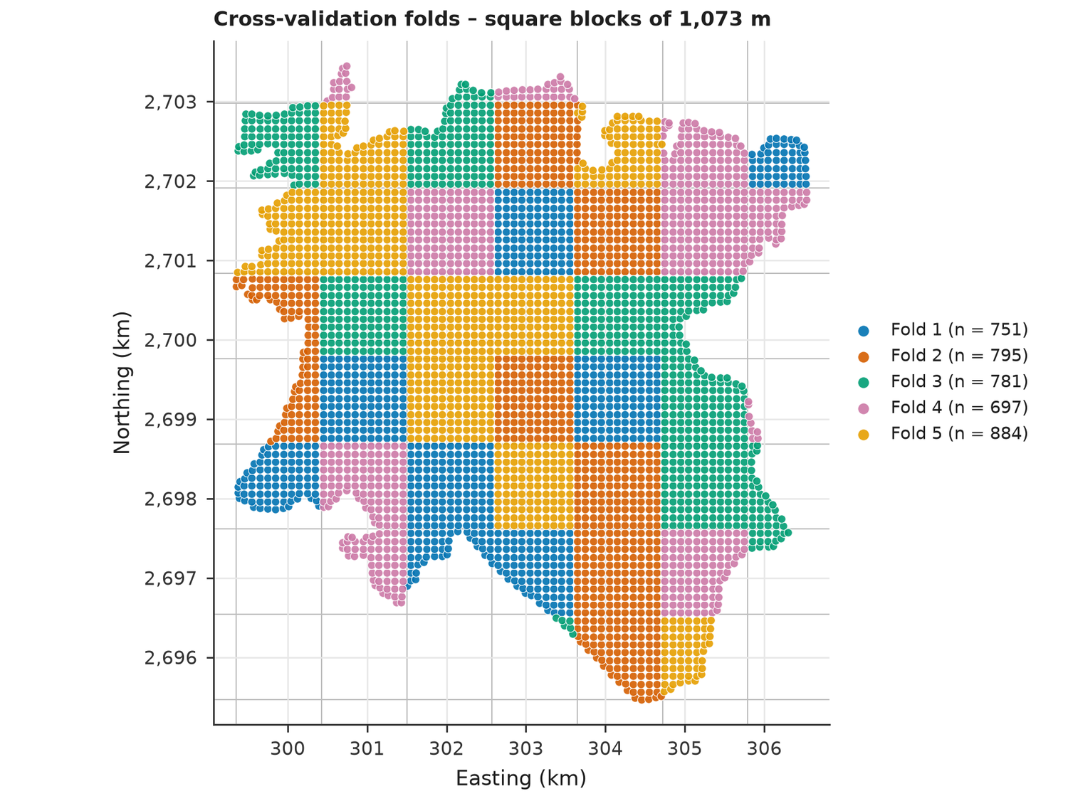
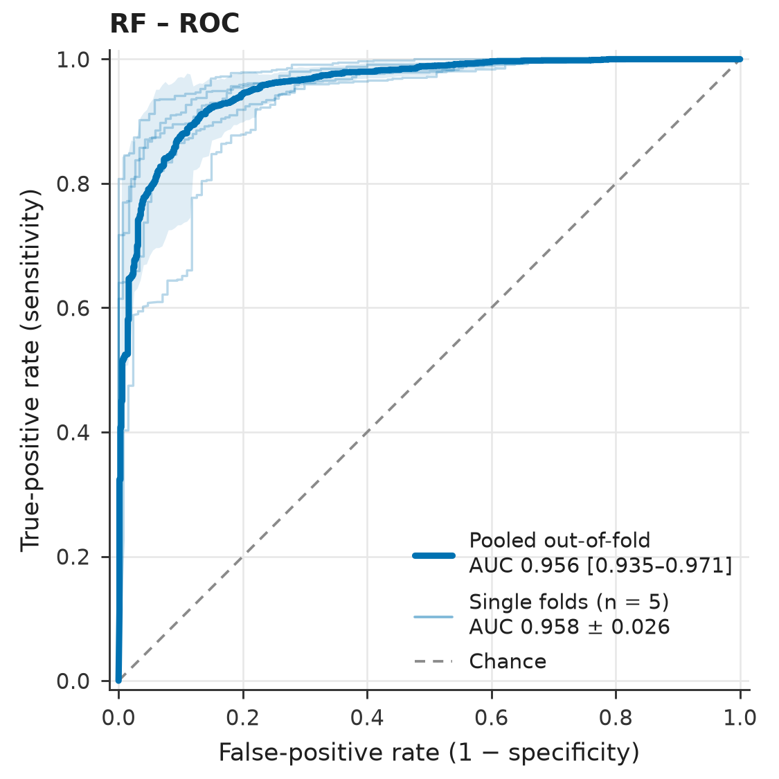
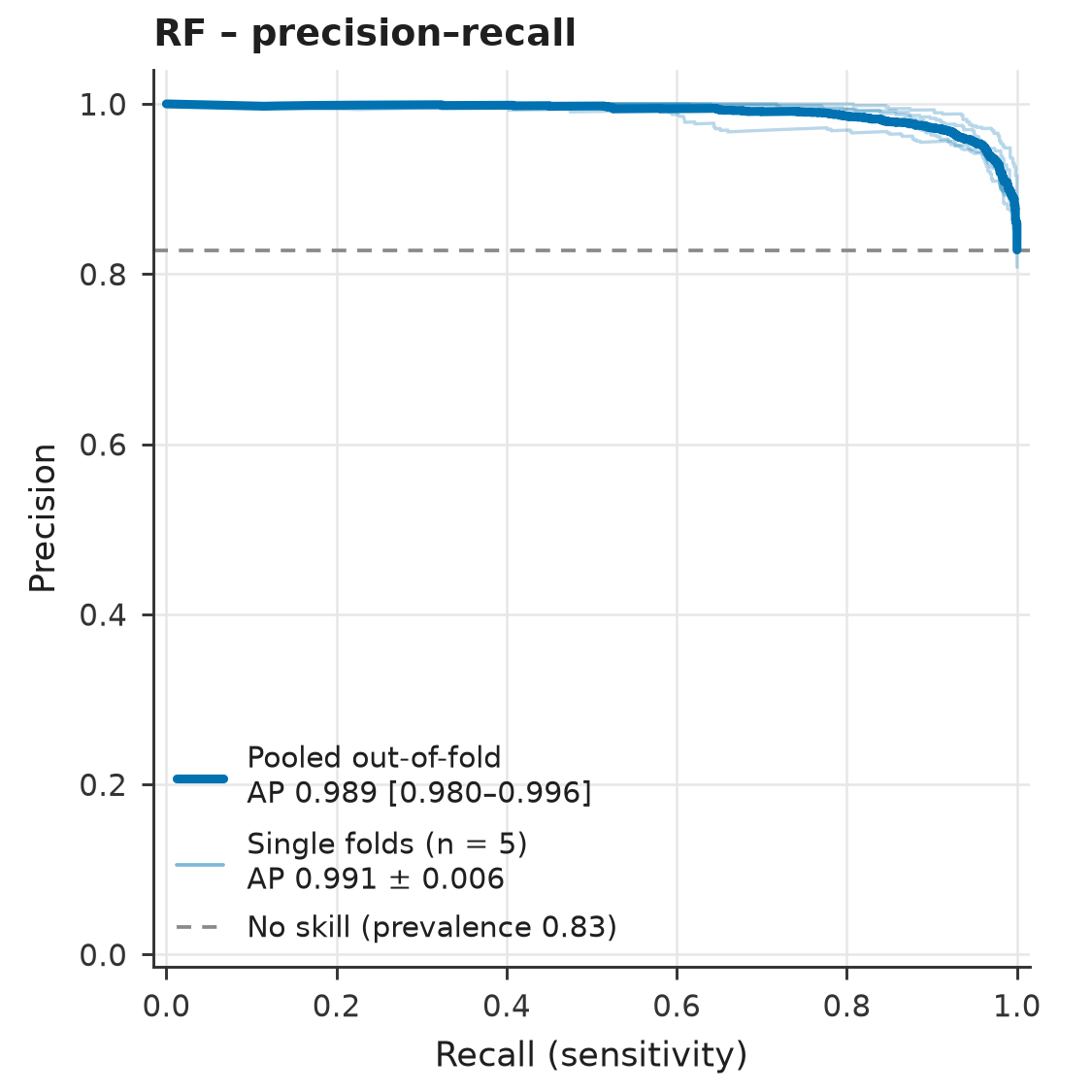
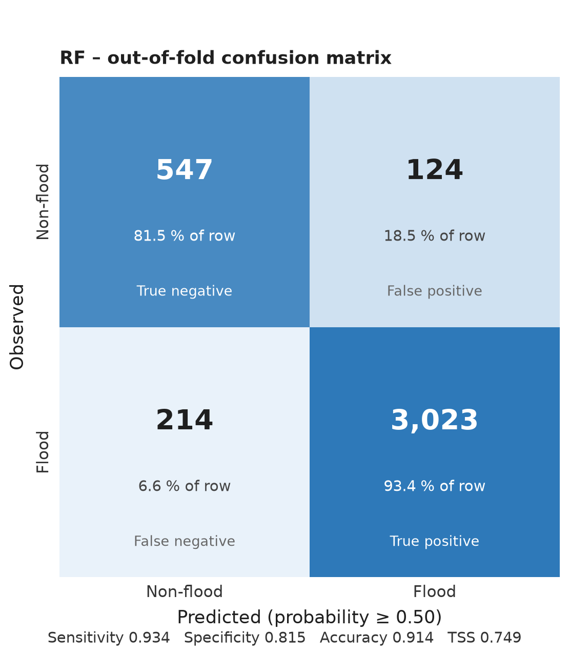
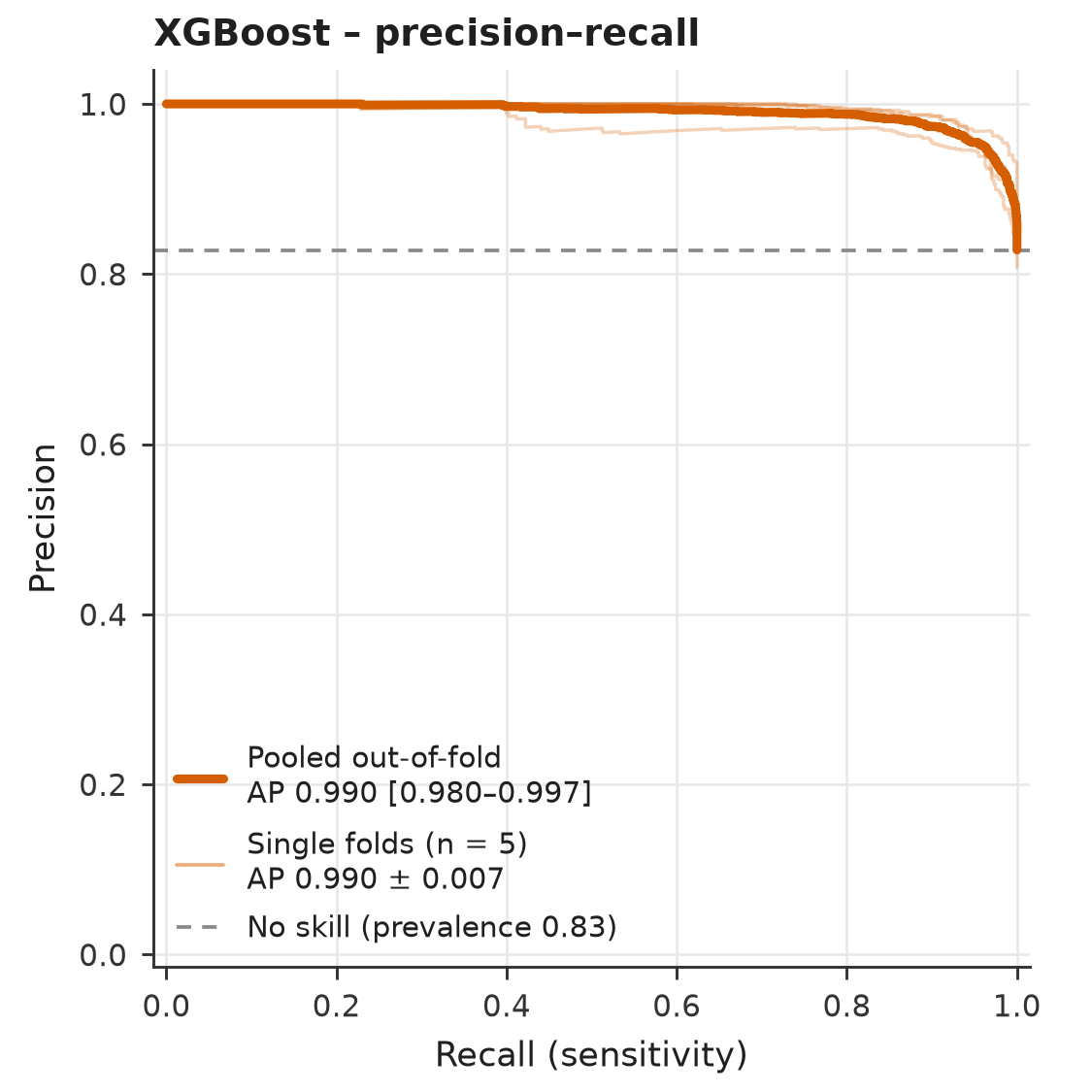
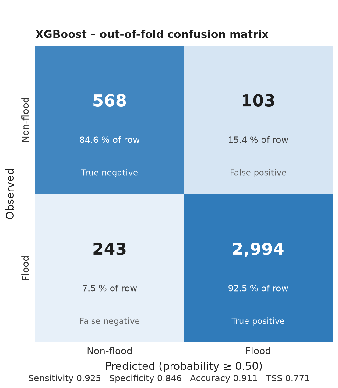
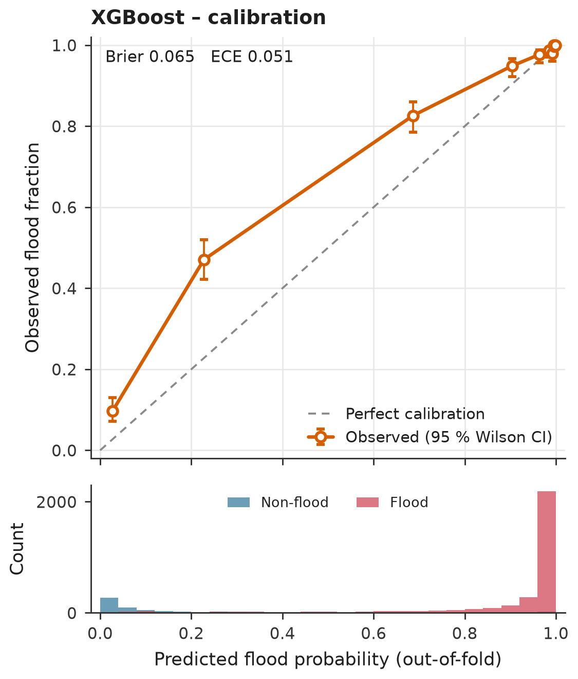
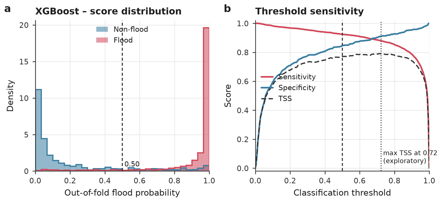
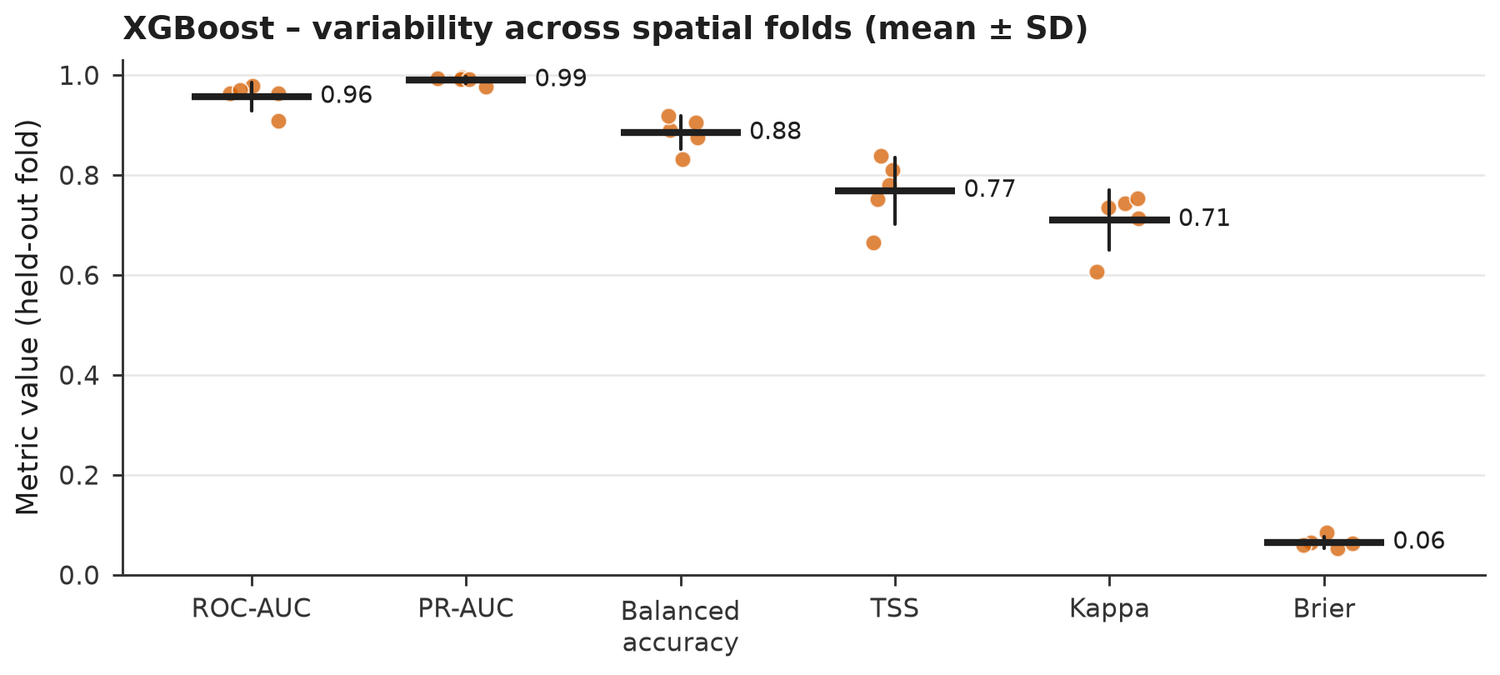
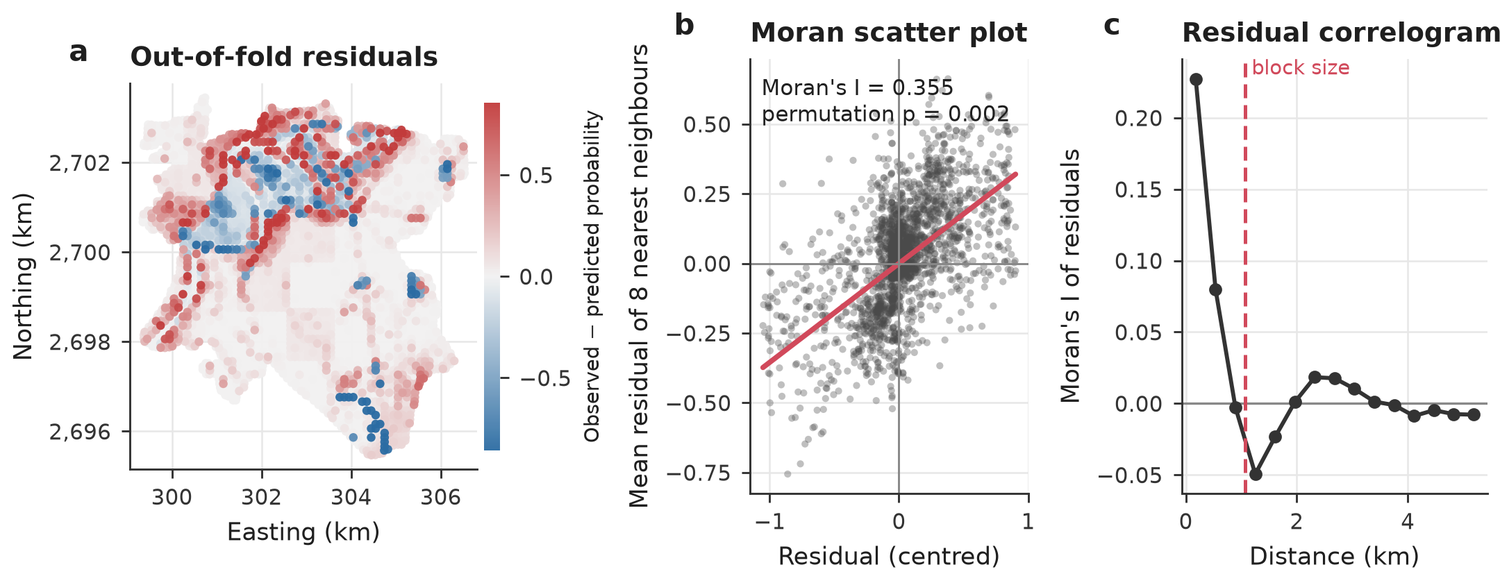
Every record is predicted by a model that did not see it or its neighbourhood. Intervals come from a cluster bootstrap over the spatial blocks.
| Model | ROC-AUC [95 % CI] | PR-AUC [95 % CI] | TSS [95 % CI] | Balanced acc. | Kappa | Brier [95 % CI] | ECE | Fold AUC mean±SD |
|---|---|---|---|---|---|---|---|---|
| RF | 0.956 [0.935–0.971] | 0.989 [0.980–0.996] | 0.749 [0.697–0.801] | 0.875 | 0.711 | 0.064 [0.044–0.083] | 0.052 | 0.958 ± 0.026 |
| XGBoost | 0.956 [0.936–0.974] | 0.990 [0.980–0.997] | 0.771 [0.718–0.824] | 0.886 | 0.713 | 0.065 [0.044–0.086] | 0.051 | 0.957 ± 0.028 |
One model at a time
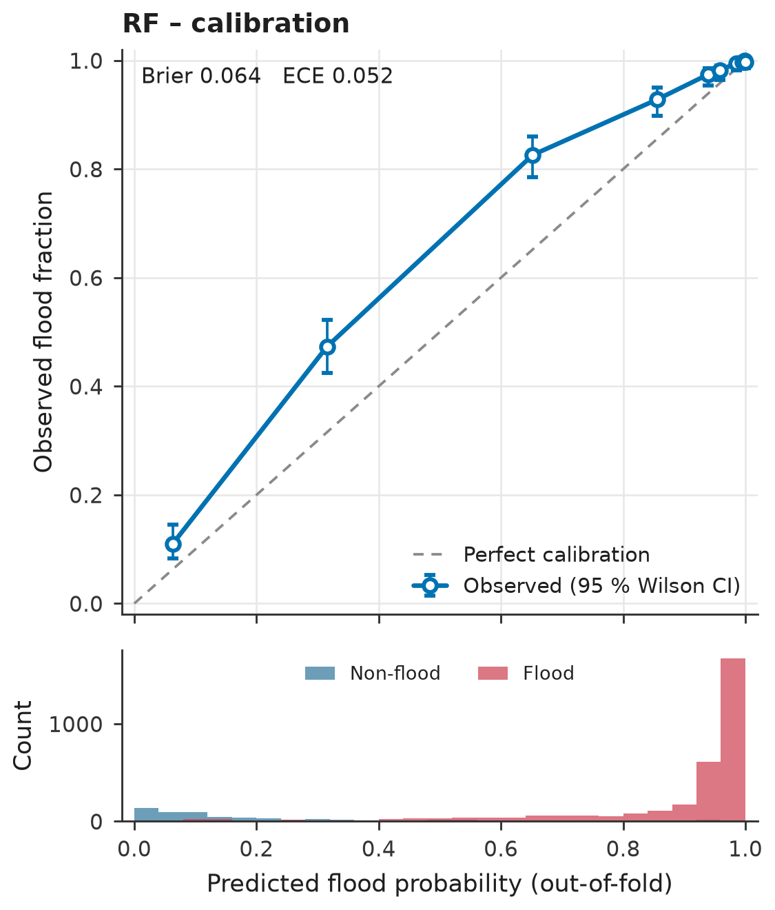
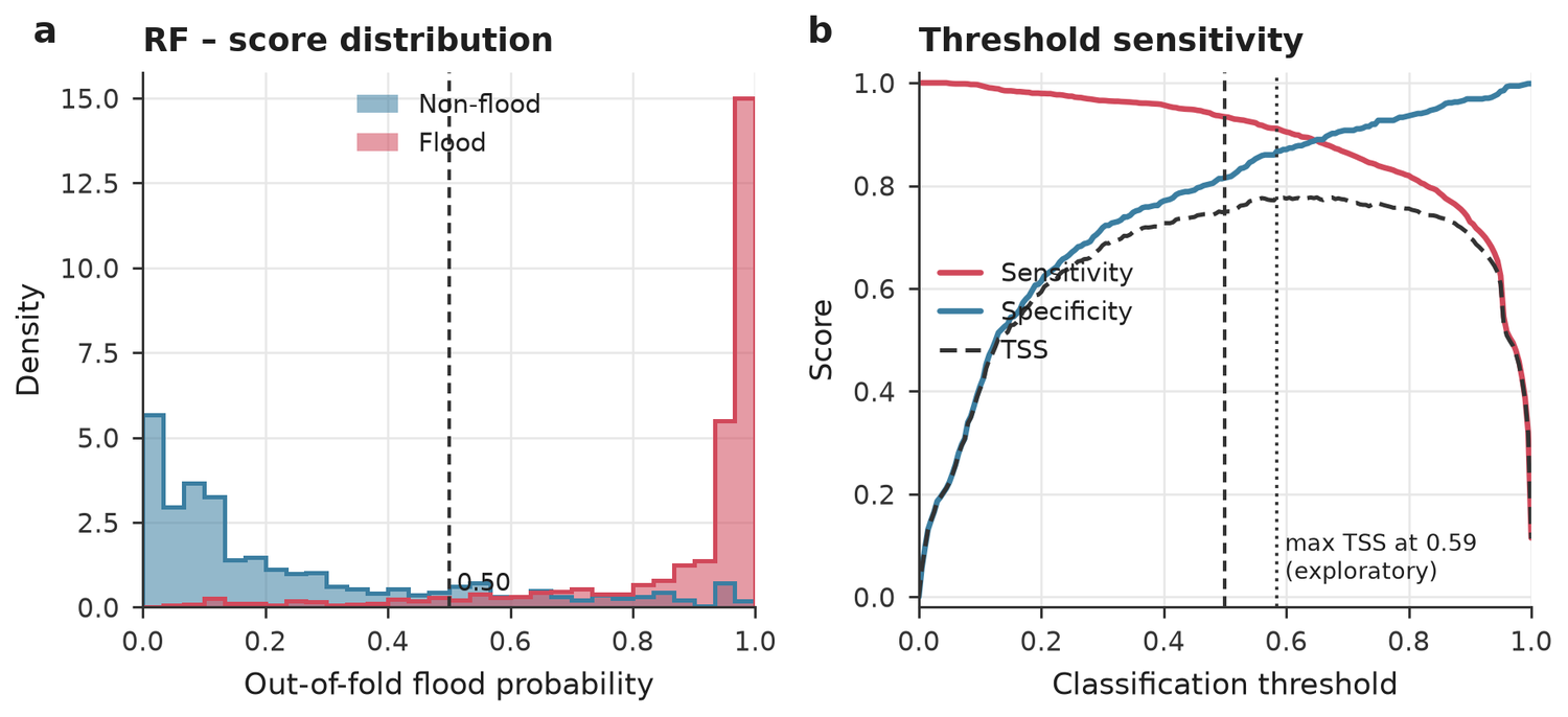
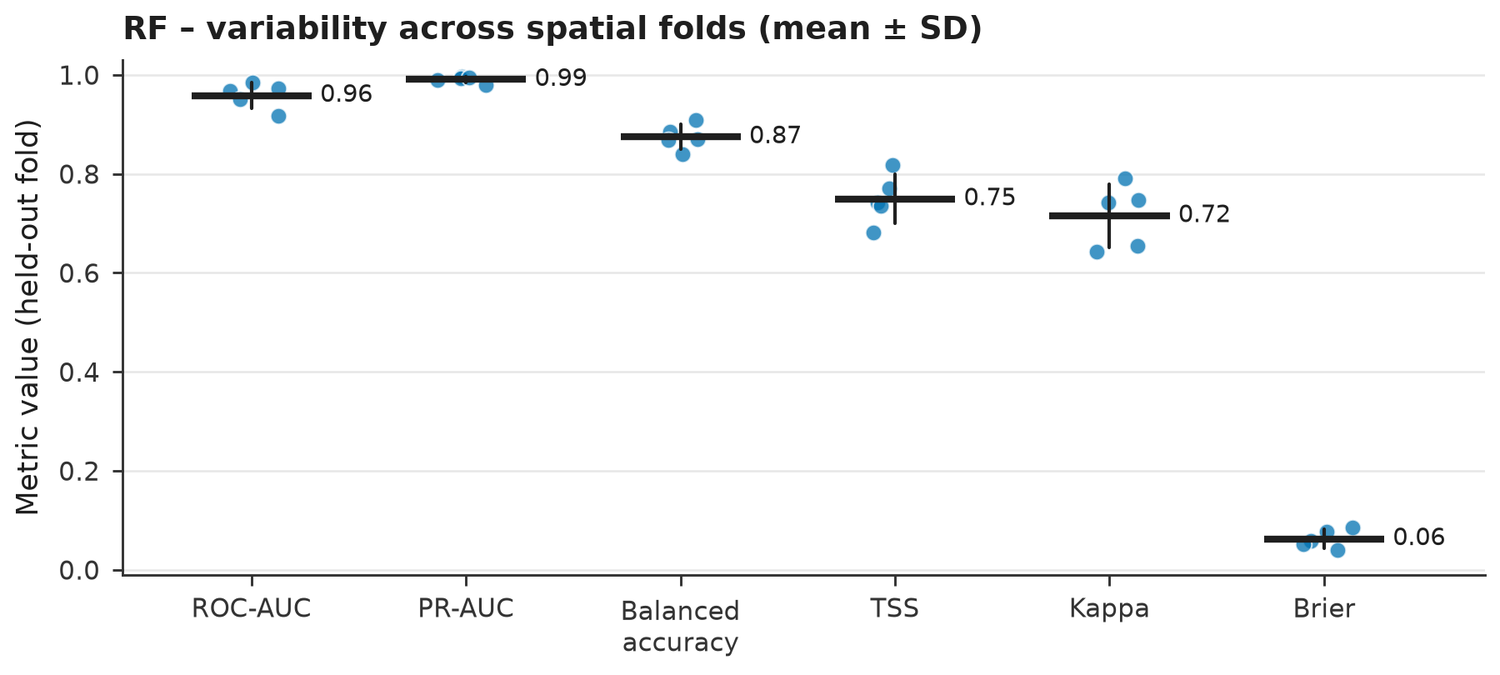
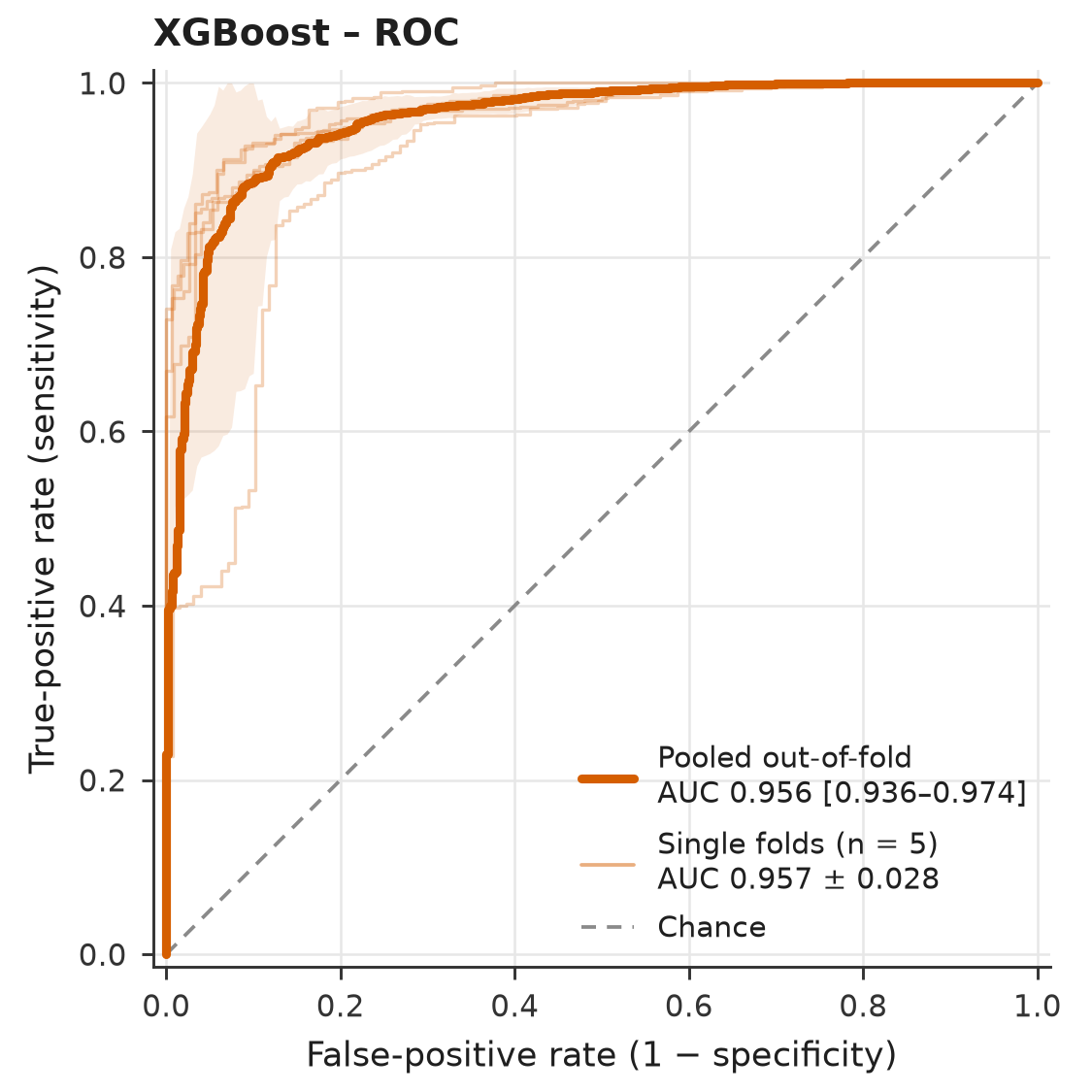
What drives the prediction
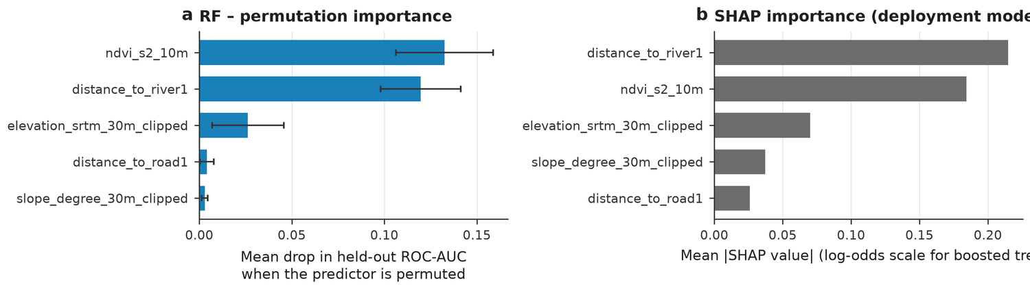
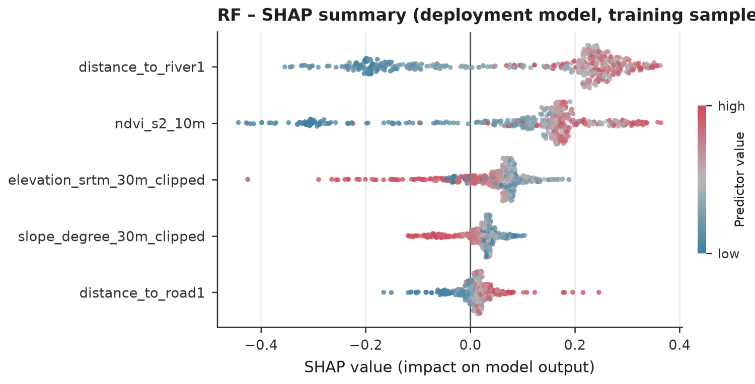
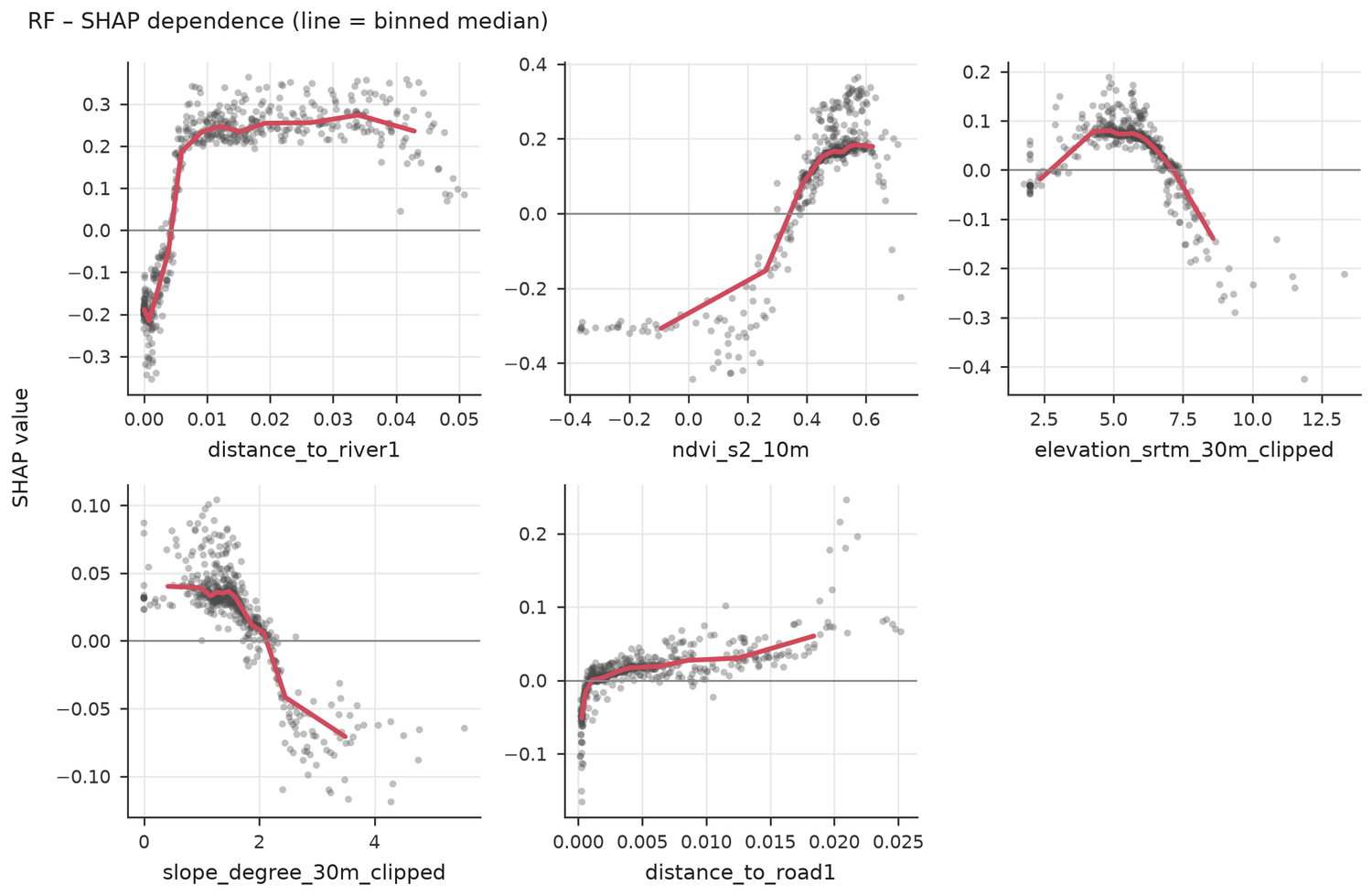
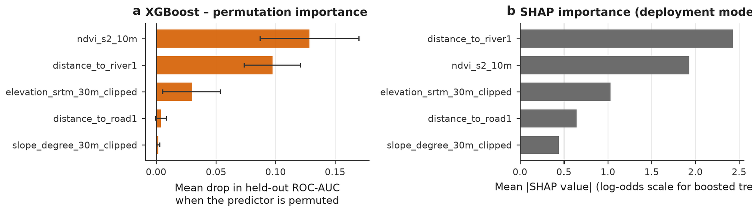
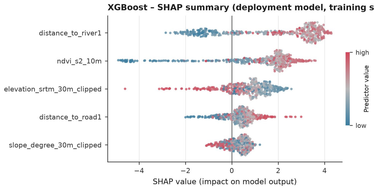
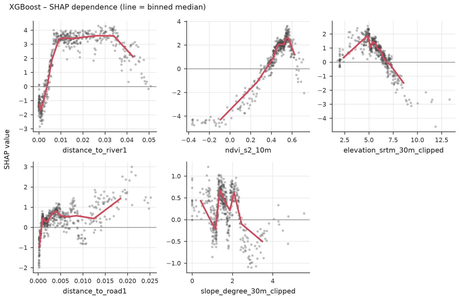
Permutation importance drops each predictor on held-out folds. SHAP shows how each value moves the prediction. Both describe the model, not cause and effect.
- Predictor 'distance_to_river1': 7 missing value(s) (median-imputed inside every fold).
- Predictor 'distance_to_road1': 7 missing value(s) (median-imputed inside every fold).
- Predictor 'elevation_srtm_30m_clipped': 3 missing value(s) (median-imputed inside every fold).
- Predictor 'slope_degree_30m_clipped': 3 missing value(s) (median-imputed inside every fold).
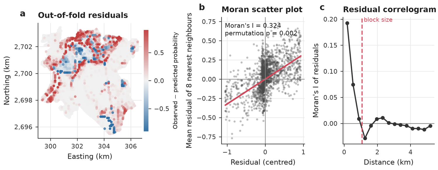
- RF: residuals are still spatially clustered (Moran I = 0.35, p = 0.002); important spatial structure may be missing from the predictors.
- XGBoost: residuals are still spatially clustered (Moran I = 0.32, p = 0.002); important spatial structure may be missing from the predictors.
Independent test
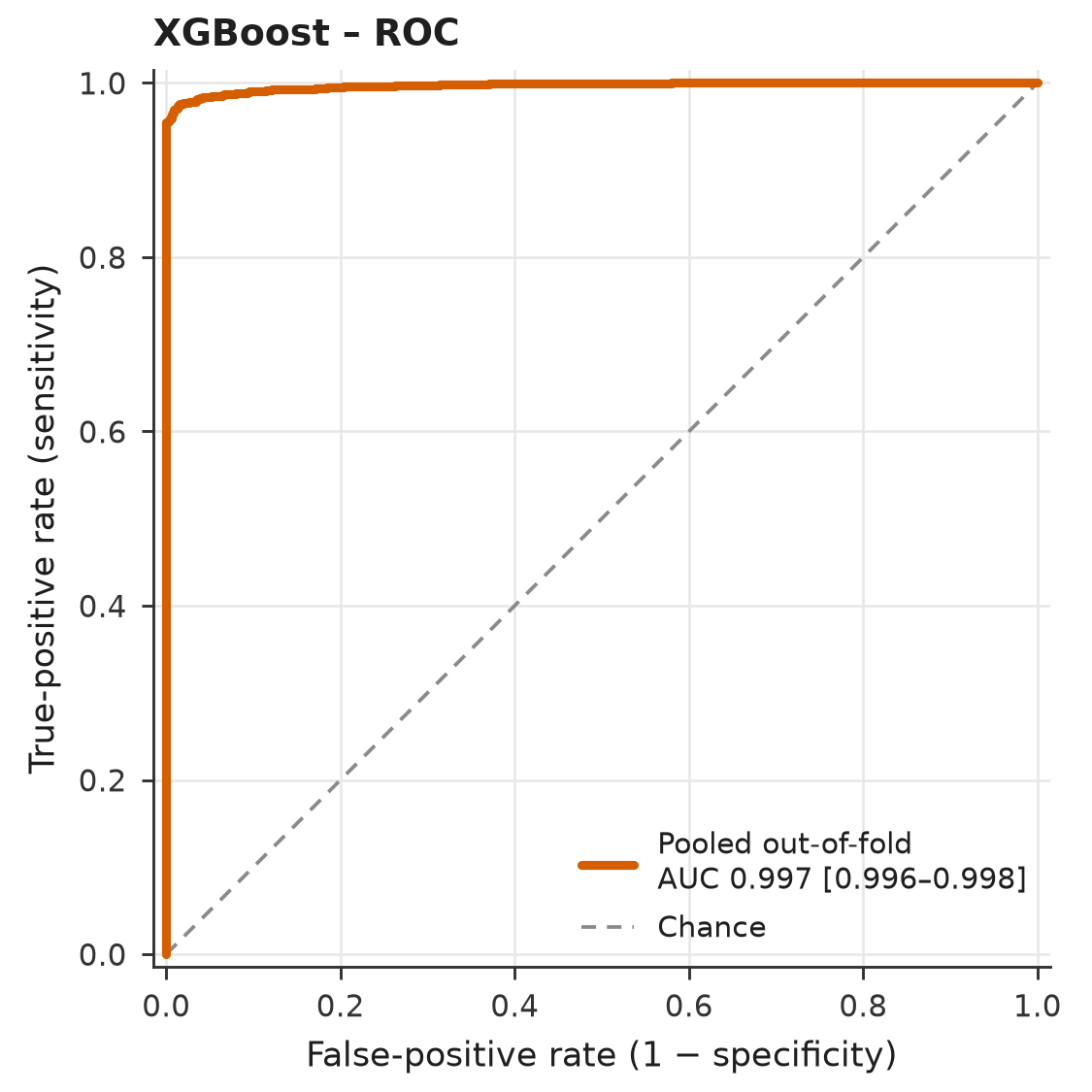
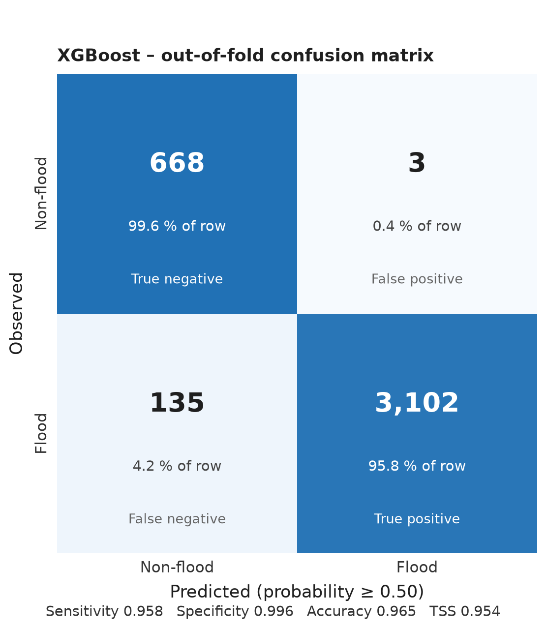
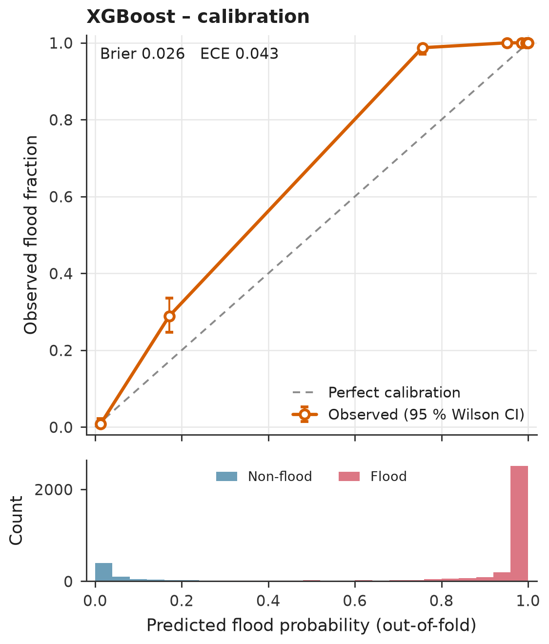
In this example the test table is the training table, so the scores below measure memory, not generalisation. The plugin detects this and refuses to call the result valid. For a real test, use another area, event or year.
| Model | ROC-AUC [95 % CI] | PR-AUC [95 % CI] | TSS | Balanced acc. | Kappa | Brier | ECE | CV ROC-AUC |
|---|---|---|---|---|---|---|---|---|
| XGBoost | 0.997 [0.996–0.998] | 0.999 [0.999–1.000] | 0.954 | 0.977 | 0.885 | 0.026 | 0.043 | 0.956 |
| RF | 0.990 [0.988–0.992] | 0.998 [0.997–0.998] | 0.895 | 0.947 | 0.818 | 0.041 | 0.062 | 0.956 |
- NOT INDEPENDENT: 100 % of the test records are identical to training records of XGBoost (same coordinates). The scores below measure how well the model remembers its training data, not how it generalises. Do not report them. Build the test table from another area, event or year.
Reading these results
This page shows one run of the plugin on 3,908 grid cells of 100 m around 24.40° N, 91.05° E. The flood label comes from a flood record raster, and the predictors are distance to river, distance to road, elevation, slope and NDVI.
The numbers are a demonstration of what the reports look like, not a finished flood study. Two limits of this run are worth knowing. Permanent water was not excluded from the training table, so the river channel is scored as a non-flood area. And the independent test used the training table, which the plugin flags as not valid. Rebuild the table with the water-exclusion option of tool 01 before you use a map for decisions.
- A predictor must be known before the flood. A layer made from the flood image leaks the answer.
- Scores are susceptibility ranks, not flood depth, return period or risk.
- Tree models do not enforce the direction you give a predictor; the direction only changes scaling.
- Check the extrapolation raster before trusting cells outside the training range.
Full reports
The complete files written by the plugin, with every figure and table.
Data check Training and validation Independent test User guide